
Kernel Methods from 2-D to 3-D
Published:
When a Line Won’t Do, Add a Dimension: Kernel Methods from 2-D to 3-D
A hands-on walkthrough with Python and R
The problem: data a straight line can’t split
Picture two groups of points on a sheet of paper: an inner ring of orange dots with an outer ring of blue dots around it. Now try to separate them with one straight line.
You can’t. Wherever you draw the line, it cuts through both rings. Yet any child could separate the groups at once by drawing a circle.
This is the basic difficulty behind a large family of machine-learning tools. Many of our best classifiers, such as the perceptron, logistic regression and the support vector machine (SVM), are linear: they separate classes with a line in 2-D, a plane in 3-D, or a hyperplane in higher dimensions. They are fast, well understood and backed by strong theory. They are also helpless against the rings.
Kernel methods keep the linear classifier and change the space it works in.
The key idea: lift the data
Suppose each point on the paper is lifted off the page, and the height of each point is its squared distance from the centre:
\[\phi(x_1, x_2) = \big(\,x_1,\;\; x_2,\;\; x_1^2 + x_2^2\,\big) = (z_1, z_2, z_3).\]- Points in the inner ring are close to the centre, so \(x_1^2 + x_2^2\) is small and they stay low.
- Points in the outer ring are far from the centre, so \(x_1^2 + x_2^2\) is large and they rise high.
The flat sheet becomes a bowl (a paraboloid). The orange points sit near the bottom and the blue points sit up on the rim, so a flat horizontal plane slides between them:
\[z_3 = c \quad\Longleftrightarrow\quad x_1^2 + x_2^2 = c .\]A plane in the lifted 3-D space, viewed from above in the original 2-D space, is a circle of radius \(\sqrt{c}\). The classifier stays linear; only the space it looks at changes.
The rest of this post builds that idea one step at a time. Each step shows the maths, then the code in Python (scikit-learn) and R (kernlab), then the output the code produced.
Setup. Python needs
numpy,matplotlibandscikit-learn. R needskernlabandscatterplot3d:install.packages(c("kernlab", "scatterplot3d")). The two languages use different random-number generators, so their datasets are similar but not identical, and their numbers differ slightly.
Step 1: Generate data that no line can separate
We draw 400 points in two noisy concentric rings: an outer ring of radius 1.0 and an inner ring of radius 0.4. Then we hold out 25% of the points for testing.
Python
import numpy as np
import matplotlib.pyplot as plt
from sklearn.datasets import make_circles
from sklearn.model_selection import train_test_split
from sklearn.svm import SVC

X, y = make_circles(n_samples=400, factor=0.4, noise=0.08, random_state=42)
X_train, X_test, y_train, y_test = train_test_split(
    X, y, test_size=0.25, random_state=42, stratify=y
)
R
library(kernlab)
library(scatterplot3d)
set.seed(42)

make_circles <- function(n = 400, factor = 0.4, noise = 0.08) {
  n_half <- n / 2
  t_out  <- runif(n_half, 0, 2 * pi)
  t_in   <- runif(n_half, 0, 2 * pi)
  X <- rbind(cbind(cos(t_out), sin(t_out)),
             factor * cbind(cos(t_in), sin(t_in)))
  X <- X + matrix(rnorm(2 * n, 0, noise), ncol = 2)
  data.frame(x1 = X[, 1], x2 = X[, 2],
             y  = factor(c(rep("outer", n_half), rep("inner", n_half))))
}

df    <- make_circles()
idx   <- sample(nrow(df), 0.75 * nrow(df))
train <- df[idx, ]
test  <- df[-idx, ]
acc   <- function(pred, truth) mean(pred == truth)
Step 2: Show that a linear classifier fails in 2-D
First we give a linear SVM the raw coordinates \((x_1, x_2)\). It searches for the best line \(w_1 x_1 + w_2 x_2 + b = 0\).
Python
svm_2d = SVC(kernel="linear", C=1.0).fit(X_train, y_train)
print(f"Linear SVM in 2-D   test accuracy: {svm_2d.score(X_test, y_test):.3f}")
R
m_2d <- ksvm(y ~ x1 + x2, data = train, kernel = "vanilladot",
             C = 1, scaled = FALSE)
cat(sprintf("Linear SVM in 2-D   test accuracy: %.3f\n",
            acc(predict(m_2d, test), test$y)))
Output
| Python | R | |
|---|---|---|
| Linear SVM in 2-D, test accuracy | 0.550 | 0.690 |
With two balanced classes, 50% is a coin flip, so the linear model has learned almost nothing. The dashed line in panel (a) of Figure 1 below shows its “best” line cutting straight through both rings. (The R figure is harder to judge because R’s random sample happens to give the line a bit more room.)
Step 3: Lift the data to 3-D with a feature map
Next we build the map \(\phi(x_1, x_2) = (x_1,\, x_2,\, x_1^2 + x_2^2)\) explicitly. The third coordinate records the thing that actually separates the classes: distance from the origin.
Python
def phi(X):
    """Map (x1, x2) -> (x1, x2, x1^2 + x2^2)."""
    return np.column_stack([X[:, 0], X[:, 1], X[:, 0] ** 2 + X[:, 1] ** 2])

Z_train, Z_test = phi(X_train), phi(X_test)
R
phi <- function(d) data.frame(z1 = d$x1, z2 = d$x2,
                              z3 = d$x1^2 + d$x2^2, y = d$y)
train3 <- phi(train)
test3  <- phi(test)
For the inner ring, \(z_3 \approx 0.4^2 = 0.16\). For the outer ring, \(z_3 \approx 1.0^2 = 1.0\). The classes now sit at clearly different heights.
Step 4: Fit a linear classifier in 3-D
We run the same linear SVM as in Step 2, this time on the lifted coordinates. It now looks for a plane:
\[w_1 z_1 + w_2 z_2 + w_3 z_3 + b = 0 .\]Python
svm_3d = SVC(kernel="linear", C=1.0).fit(Z_train, y_train)
print(f"Linear SVM in 3-D   test accuracy: {svm_3d.score(Z_test, y_test):.3f}")

w, b = svm_3d.coef_[0], svm_3d.intercept_[0]
print(f"Separating plane: {w[0]:+.3f} z1 {w[1]:+.3f} z2 {w[2]:+.3f} z3 {b:+.3f} = 0")
R
m_3d <- ksvm(y ~ z1 + z2 + z3, data = train3, kernel = "vanilladot",
             C = 1, scaled = FALSE)
cat(sprintf("Linear SVM in 3-D   test accuracy: %.3f\n",
            acc(predict(m_3d, test3), test3$y)))

# kernlab's decision function is w.z - b, so the plane is w.z = b
w <- colSums(coef(m_3d)[[1]] * xmatrix(m_3d)[[1]])
b <- b(m_3d)
cat(sprintf("Separating plane: %+.3f z1 %+.3f z2 %+.3f z3 = %+.3f\n",
            w[1], w[2], w[3], b))
Output (Python)
Linear SVM in 3-D   test accuracy: 1.000
Separating plane: +0.003 z1 +0.123 z2 -4.230 z3 +2.165 = 0
Output (R)
Linear SVM in 3-D   test accuracy: 1.000
Separating plane: +0.030 z1 +0.008 z2 +3.693 z3 = +2.026
Accuracy jumps from roughly chance to 100% in both languages. The only change was adding one coordinate.
Step 5: Map the plane back to 2-D and see a circle
Substituting \(z = \phi(x)\) into the plane gives the boundary in the original coordinates:
\[w_1 x_1 + w_2 x_2 + w_3 (x_1^2 + x_2^2) + b = 0 .\]With \(w_3 \neq 0\) this is a circle. Now read off the fitted numbers:
- Python: the \(z_1\) and \(z_2\) coefficients (0.003 and 0.123) are tiny next to \(z_3\) (−4.230), so the plane is almost horizontal. It sits at \(z_3 \approx 2.165 / 4.230 \approx 0.51\), which is a circle of radius \(\sqrt{0.51} \approx 0.72\).
- R: the plane sits at \(z_3 \approx 2.026 / 3.693 \approx 0.55\), which is a circle of radius \(\sqrt{0.55} \approx 0.74\).
Both radii fall between the inner ring (0.4) and the outer ring (1.0), roughly where you would draw the circle by hand.
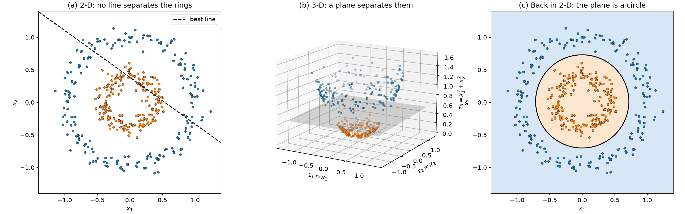
(a) The best straight line fails in 2-D. (b) After the lift, a flat plane separates the classes. (c) Pulled back to 2-D, the plane becomes a circle.
Code that draws the figures
Python
colors = np.where(y == 1, "tab:orange", "tab:blue")
fig = plt.figure(figsize=(16, 5))

# (a) original 2-D data with the failed linear boundary
ax1 = fig.add_subplot(1, 3, 1)
ax1.scatter(X[:, 0], X[:, 1], c=colors, s=14, edgecolor="k", linewidth=0.3)
xs = np.linspace(-1.4, 1.4, 50)
w2, b2 = svm_2d.coef_[0], svm_2d.intercept_[0]
if abs(w2[1]) > 1e-9:
    ax1.plot(xs, -(w2[0] * xs + b2) / w2[1], "k--", label="best line")
    ax1.legend(loc="upper right")
ax1.set(xlim=(-1.4, 1.4), ylim=(-1.4, 1.4), aspect="equal",
        title="(a) 2-D: no line separates the rings", xlabel="$x_1$", ylabel="$x_2$")

# (b) lifted 3-D data with the separating plane
ax2 = fig.add_subplot(1, 3, 2, projection="3d")
Z = phi(X)
ax2.scatter(Z[:, 0], Z[:, 1], Z[:, 2], c=colors, s=10, edgecolor="k", linewidth=0.2)
gx, gy = np.meshgrid(np.linspace(-1.3, 1.3, 20), np.linspace(-1.3, 1.3, 20))
gz = -(w[0] * gx + w[1] * gy + b) / w[2]
ax2.plot_surface(gx, gy, gz, alpha=0.25, color="gray")
ax2.set(title="(b) 3-D: a plane separates them",
        xlabel="$z_1=x_1$", ylabel="$z_2=x_2$", zlabel="$z_3=x_1^2+x_2^2$")
ax2.view_init(elev=15, azim=-60)

# (c) the plane pulled back into 2-D becomes a circle
ax3 = fig.add_subplot(1, 3, 3)
gx2, gy2 = np.meshgrid(np.linspace(-1.4, 1.4, 300), np.linspace(-1.4, 1.4, 300))
grid = np.column_stack([gx2.ravel(), gy2.ravel()])
dec = svm_k.decision_function(grid).reshape(gx2.shape)   # svm_k is built in Step 6
ax3.contourf(gx2, gy2, dec, levels=[-100, 0, 100],
             colors=["#cfe2f3", "#fde0c5"], alpha=0.8)
ax3.contour(gx2, gy2, dec, levels=[0], colors="k", linewidths=1.5)
ax3.scatter(X[:, 0], X[:, 1], c=colors, s=14, edgecolor="k", linewidth=0.3)
ax3.set(aspect="equal", title="(c) Back in 2-D: the plane is a circle",
        xlabel="$x_1$", ylabel="$x_2$")

plt.tight_layout()
plt.savefig("kernel_lift_python.png", dpi=150)
plt.show()
R
cols <- ifelse(df$y == "inner", "darkorange", "steelblue")
png("kernel_lift_R.png", width = 1800, height = 600, res = 120)
par(mfrow = c(1, 3))

# (a) original 2-D data
plot(df$x1, df$x2, col = cols, pch = 19, cex = 0.7, asp = 1,
     xlab = expression(x[1]), ylab = expression(x[2]),
     main = "(a) 2-D: no line separates the rings")

# (b) lifted 3-D data with the separating plane  z3 = (b - w1 z1 - w2 z2) / w3
d3 <- phi(df)
s3 <- scatterplot3d(d3$z1, d3$z2, d3$z3, color = cols, pch = 19,
                    cex.symbols = 0.6, angle = 55,
                    xlab = "z1 = x1", ylab = "z2 = x2", zlab = "z3 = x1^2 + x2^2",
                    main = "(b) 3-D: a plane separates them")
s3$plane3d(Intercept = b / w[3], x.coef = -w[1] / w[3], y.coef = -w[2] / w[3],
           col = "gray30", lty = "dashed")

# (c) the plane pulled back into 2-D becomes a circle  (m_k is built in Step 6)
gs   <- seq(-1.4, 1.4, length.out = 120)
grid <- as.matrix(expand.grid(x1 = gs, x2 = gs))
dec  <- matrix(predict(m_k, grid, type = "decision"), nrow = length(gs))
cls  <- matrix(predict(m_k, grid) == "inner", nrow = length(gs))
image(gs, gs, cls, col = c("#cfe2f3", "#fde0c5"), asp = 1,
      xlab = expression(x[1]), ylab = expression(x[2]),
      main = "(c) Back in 2-D: the plane is a circle")
contour(gs, gs, dec, levels = 0, add = TRUE, lwd = 2, drawlabels = FALSE)
points(df$x1, df$x2, col = cols, pch = 19, cex = 0.7)

dev.off()
Step 6: The kernel trick, or lifting without lifting
Building \(\phi(\mathbf{x})\) explicitly is fine for one extra dimension. But what if the right space has 50 dimensions, or 5,000, or infinitely many? That is where the kernel comes in.
Why inner products are all we need
When a linear SVM is written in its dual form, the data appear only through inner products between pairs of points:
\[\max_{\alpha}\; \sum_i \alpha_i \;-\; \tfrac12 \sum_{i,j} \alpha_i \alpha_j\, y_i y_j\, \langle \phi(\mathbf{x}_i), \phi(\mathbf{x}_j) \rangle \quad \text{s.t.}\quad 0 \le \alpha_i \le C,\;\; \sum_i \alpha_i y_i = 0,\]and new points are classified with
\[f(\mathbf{x}) = \operatorname{sign}\Big( \sum_i \alpha_i y_i \,\langle \phi(\mathbf{x}_i), \phi(\mathbf{x}) \rangle + b \Big).\]The coordinates \(\phi(\mathbf{x})\) are never needed on their own, only the inner products between them.
Computing the inner product directly
A kernel returns that inner product using only the original coordinates. For our lift:
\[\begin{aligned} \langle \phi(\mathbf{x}), \phi(\mathbf{x}') \rangle &= x_1 x_1' + x_2 x_2' + (x_1^2 + x_2^2)(x_1'^2 + x_2'^2) \\ &= \mathbf{x}\cdot\mathbf{x}' \;+\; \|\mathbf{x}\|^2 \,\|\mathbf{x}'\|^2 , \end{aligned}\]so
\[\boxed{K(\mathbf{x}, \mathbf{x}') = \mathbf{x}\cdot\mathbf{x}' + \|\mathbf{x}\|^2 \|\mathbf{x}'\|^2}\]In code
We write this kernel as a function and check numerically that it equals the inner product of the lifted vectors. Then we give it to the SVM together with the original 2-D data. Note that phi is never called when fitting.
Python (scikit-learn wants a function that returns the full Gram matrix between two sets of points)
def circle_kernel(A, B):
    """K(a, b) = a.b + ||a||^2 ||b||^2  (Gram matrix for all pairs)."""
    return A @ B.T + np.outer((A ** 2).sum(axis=1), (B ** 2).sum(axis=1))

# Sanity check: kernel equals the inner product of the lifted vectors
assert np.allclose(circle_kernel(X_train[:5], X_train[:5]),
                   phi(X_train[:5]) @ phi(X_train[:5]).T)

svm_k = SVC(kernel=circle_kernel, C=1.0).fit(X_train, y_train)   # raw 2-D data
print(f"Kernel-trick SVM    test accuracy: {svm_k.score(X_test, y_test):.3f}")
agree = np.mean(svm_k.predict(X_test) == svm_3d.predict(Z_test))
print(f"Agreement between explicit-lift and kernel-trick predictions: {agree:.3f}")
R (kernlab wants a function of two vectors with class "kernel")
circle_kernel <- function(x, y) sum(x * y) + sum(x^2) * sum(y^2)
class(circle_kernel) <- "kernel"

# Sanity check: kernel equals the inner product of the lifted vectors
a <- c(0.3, -0.7); bb <- c(1.1, 0.2)
stopifnot(isTRUE(all.equal(circle_kernel(a, bb),
                           sum(c(a, sum(a^2)) * c(bb, sum(bb^2))))))

Xtr <- as.matrix(train[, c("x1", "x2")])
Xte <- as.matrix(test[, c("x1", "x2")])
m_k <- ksvm(Xtr, train$y, kernel = circle_kernel, C = 1, scaled = FALSE)
pred_k <- predict(m_k, Xte)
cat(sprintf("Kernel-trick SVM    test accuracy: %.3f\n", acc(pred_k, test$y)))
cat(sprintf("Agreement between explicit-lift and kernel-trick predictions: %.3f\n",
            acc(pred_k, predict(m_3d, test3))))
Output (identical in both languages)
Kernel-trick SVM    test accuracy: 1.000
Agreement between explicit-lift and kernel-trick predictions: 1.000
The sanity check passes, and the kernel SVM agrees with the explicit 3-D SVM on every test point. It is the same model; we simply never built the third coordinate. The circular boundary in panel (c) of both figures was drawn from this kernel model.
Step 7: Compare with a general-purpose kernel
We designed the circle kernel with knowledge of the data’s shape. In practice people often use the Gaussian (RBF) kernel \(K(\mathbf{x},\mathbf{x}') = \exp(-\gamma\|\mathbf{x}-\mathbf{x}'\|^2)\), whose implicit feature space is infinite-dimensional.
Python
svm_rbf = SVC(kernel="rbf", gamma="scale", C=1.0).fit(X_train, y_train)
print(f"RBF-kernel SVM      test accuracy: {svm_rbf.score(X_test, y_test):.3f}")
R
m_rbf <- ksvm(Xtr, train$y, kernel = "rbfdot", C = 1)
cat(sprintf("RBF-kernel SVM      test accuracy: %.3f\n",
            acc(predict(m_rbf, Xte), test$y)))
Output
RBF-kernel SVM test accuracy: 1.000
RBF also solves the problem, and it does so without being told that “distance from the centre” is what matters. The price is a less interpretable boundary: we can no longer read a single radius off the fitted model.
Results summary
| Model | Space the classifier works in | Python test accuracy | R test accuracy |
|---|---|---|---|
| Linear SVM | original 2-D | 0.550 | 0.690 |
| Linear SVM on \(\phi(\mathbf{x})\) | explicit 3-D | 1.000 | 1.000 |
| SVM with circle kernel | implicit 3-D (kernel trick) | 1.000 | 1.000 |
| SVM with RBF kernel | implicit ∞-D | 1.000 | 1.000 |
A zoo of kernels
The kernel trick turns “choose a feature space” into “choose a similarity function”:
| Kernel | Formula | Implicit feature space |
|---|---|---|
| Linear | \(\mathbf{x}\cdot\mathbf{x}'\) | the original space (no lift) |
| Our “circle” kernel | \(\mathbf{x}\cdot\mathbf{x}' + |\mathbf{x}|^2|\mathbf{x}'|^2\) | 3-D (the paraboloid lift) |
| Polynomial, degree \(d\) | \((\mathbf{x}\cdot\mathbf{x}' + c)^d\) | all monomials up to degree \(d\) |
| Gaussian / RBF | \(\exp\!\big(-\gamma\,|\mathbf{x}-\mathbf{x}'|^2\big)\) | infinite-dimensional |
Evaluating \(K\) costs about the same whether the hidden space has 3 dimensions or infinitely many.
What makes a valid kernel? Not every function of two points is an inner product in disguise. Mercer’s condition gives the test: $K$ must be symmetric, and every Gram matrix \(G_{ij} = K(\mathbf{x}_i, \mathbf{x}_j)\) must be positive semi-definite. When this holds, a feature space (formally, a reproducing kernel Hilbert space) is guaranteed to exist, even if we never write it out.
Implementation notes
- Scaling. The circle kernel depends on distance from the origin, so the data must be centred. The R code sets
scaled = FALSEbecause kernlab’s automatic scaling would change the geometry. For RBF kernels, standardising features is usually a good idea. - Hyperparameters.
Ctrades a wide margin against training errors. For RBF,gammacontrols how local each point’s influence is. Tune both with cross-validation. - Cost. Kernel methods work with an $n \times n$ Gram matrix, so training cost grows roughly between $O(n^2)$ and $O(n^3)$. For large datasets, random Fourier features or the Nyström method are common approximations.
Beyond SVMs
The same trick applies to any algorithm that can be written purely in terms of inner products: kernel ridge regression, Gaussian process regression, kernel PCA, kernel k-means and spectral clustering. The pattern is always the one we used for the rings: map to a space where the problem is linear, solve it there, and let the kernel do the mapping implicitly.
Takeaways
- A linear classifier can only draw flat boundaries, and many real problems are not flatly separable (Step 2: accuracy near chance).
- A feature map $\phi$ lifts the data into a space where a flat boundary may work. Adding \(z_3 = x_1^2 + x_2^2\) turned the rings into a bowl that a plane could split (Steps 3–4: 100% accuracy).
- A flat boundary in the lifted space is a curved boundary in the original space. Here the plane became a circle of radius about 0.72 (Step 5).
- The kernel trick replaces \(\langle\phi(\mathbf{x}),\phi(\mathbf{x}')\rangle$ with $K(\mathbf{x},\mathbf{x}')\), so we get the lift without computing it (Step 6: 100% agreement with the explicit lift).
- Choosing a kernel means choosing a notion of similarity, and that is where domain knowledge enters (Step 7).
Try it yourself: change factor to move the rings closer together, raise noise until they overlap, or replace the circle kernel with the polynomial kernel \((\mathbf{x}\cdot\mathbf{x}' + 1)^2\) and compare the boundaries.